Lab Background

The purpose of this week's lab was to perform grid-based localization on our robot running in simulation using a Bayes Filter.

Lab Tasks

The first function I implemented for this lab was compute_control(). The compute_control() function takes the odometry estimated current and previous robot positions at timestep t and t-1 respectively, and returns the control input performed to move between these two poses.

The odometry motion model, as illustrated below in lecture:

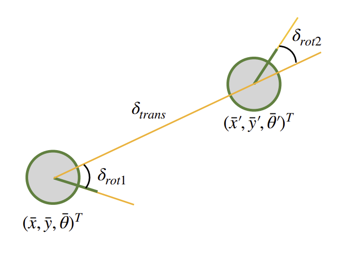
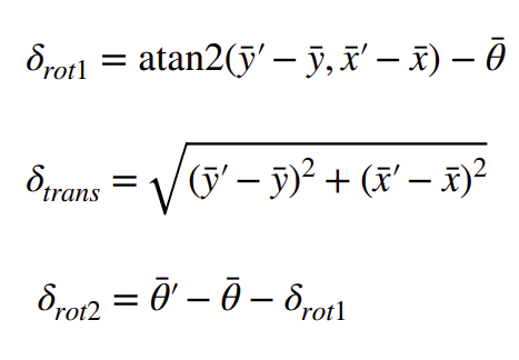
consists of 3 components: an initial rotation \( \delta_{\text{rot1}} \), a translation \( \delta_{\text{trans}} \), and a final rotation \( \delta_{\text{rot2}} \).

Using trigonometry, we can derive equations to solve for these 3 components from the given poses as shown in class:

Later, we will use these control inputs as part of the prediction step of the Bayes filter to update the belief distribution based on the robot's movement.

Next, I implemented the odom_motion_model() function. odom_motion_model() first computes \( \hat{u} \), the control input from the current and previous odomotry poses, and then computes the probability that the robot transitioned from its previous pose to the current pose given that control input.

Next, I implemented the prediction_step() function.

The prediction_step() function uses the odometry motin model to update the robot's belief of where it could be based on its movements.

We first start by initializing an empty grid with the same dimensions as our map to store our predicted belief in its position.

We then iterate through all previous poses within the grid. These poses represent the robot's possible locations in the grid from the prior timestep

For each previous pose with a belief greater than 0.0001, we loop through all possible current poses.

For each previous pose and current pose pair , we can compute the transition probability as described by the odom_motion_model() function that we implemented earlier, to estimate the likelihood that the robot moved from previous to current pose given the control input.

Multiplying this probability by the belief at the previous pose, accumulating it onto the belief at the current pose, and normalizing across the grid, we can generate a probability distribution, where each cell in the grid represents the likelihood for the robot being in that state.

Important to note is that the threshold parameter of 0.0001 is set to save on computation by excluding poses with very low probability.

The threshold value of 0.0001 was selected through trial and error to balance accuracy and compute time.

The sensor_model() function takes a series of observations within a cell, and returns the likelihood of each sensor measurement occuring given a sensor standard deviatio of sigma.

Lastly, to complete the Bayes Filter, I implemented the update_step() function. The update step refines the robot’s predicted belief (computed during the prediction step) by incorporating current sensor measurements. Using the sensor model, we compute the likelihood of each possible pose given the observations. By multiplying this likelihood with the predicted belief and normalizing the result, we obtain an updated probability distribution that represents the robot's corrected belief about its position.

The last step in the lab was to run the Bayes Filter on the given sample trajectory. In the video below, the odometry is plotted in red, the ground truth in green, and the Bayes filter corrected belief in light blue.

As we can see, despite the odometry being wildly inaccurate, the most probable state given by the Bayes filter very closely matches the ground truth trajectory.

My inference for when the Bayes Filter works best is in areas where the robot is closest to the walls, and this hypothesis is reflected in the results shown below. This is likely due to sensor measurements being more consistent and reliable at short distances, as opposed to when the robot is located further away from any obstacles.

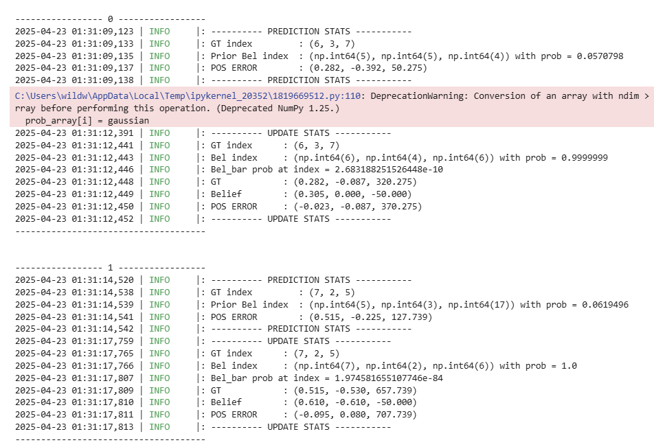
Lastly, I've attached a screenshot of the outputted most probable state after each iteration of the Bayes Filter alongside the ground truth:

Collaboration Statement

I referenced Nila Narayan's website for this lab.