Lab Tasks

Orientation Control: Tune your PID orientation controller to allow your robot to do on-axis turns in small, accurate increments. If you choose this option, you can score up to 7.5 points in this lab.

I started this week's lab by modifying my angular PD control loop from Lab 6 to make a full 360 degree rotation in small increments while simultaneously capturing and recording ToF measurements.

To accomplish this, I first modified my control loop to include an incrementing function that iterates to the next setpoint on a given delay interval. As shown in the snippet below, the function iterates through setpoint angles of 0 to 360 in 15 degree increments:

For this loop to work, I needed to make a slight modification to my get_yaw() function, which returns the current yaw angle calculated by the DMP.

Previously, this function returned values from a range of {-180,180}, but to align with my desired angles of 0 to 360, I needed to add a correction of 360 degrees to negative angles to correctly map values into the (0,360) degree range.

Lastly, I needed to extend my implementation for the pid_to_pwm_angular() function to include a check to take ToF measurements only when the robot has settled at a setpoint.

By implementing this check, the robot only sets the ToF measurement flag when it has settled at its new setpoint.

Altogether, this approach allowed me to reuse the majority of my angular PD controller code to cycle through setpoints on a timed interval while collecting ToF recordings.

Please upload a video that shows if your robot turns (roughly) on axis.

Additionally, I've also attached a video of my mapping program successfully running on the robot at 3 different measurement locations:

As can be seen in the video above, the first run of the controller at the (-3,-2) measurement point has an initial overshoot and overcorrection, resulting in the robot making a full rotation before settling at its new setpoint, which resulted in the robot drifting slightly out of frame.

I was still able to use the measurements from this run by adding a manual offset of +.5 ft in the x axis for datapoints recorded at this location to account for the altered measurement point. I'm still unsure as to what caused this error in the first place, but I speculate that this was likely due to my controller gains or the varying floor conditions from measurement point to measurement point. As seen in the clip, this problem resolved itself in all later scans.

Given any potential drift in your sensor, the size and accuracy of your increments, and how reliably your robot turns on axis, reason about the average and maximum error of your map if you were to do an on-axis turn in the middle of a 4x4m square, empty room.

As I had chosen to use the DMP instead of the raw angular data from the drift-prone gryoscope, I was fairly confident that the potential drift from the sensor was relatively negligble.

Instead, the accuracy and reliability of my robots turns, as well as the ranging error in the ToF sensors were a much greater concern for me. The size of my turning increments was 15 degrees, and my PD controller code allowed for 5 degrees of error in either direction from the setpoint. Additionally, the ranging error in the ToF sensors in long distance mode was given to be approximately +- 20mm.

Assuming these error conditions and the fact that my robot was able to make relatively on-axis turns, we can simplify our problem to use basic trigonometry to roughly estimate the maximum error of the map.

If we have an angular error of +-5 degrees, and a distance from the wall of 2 meters in a 4mx4m arena (if the robot is placed in the middle), with an additional + 20mm to account for maximum ranging error of the ToF sensor,

We can then solve for the maximum lateral error along the edges of the map using the following formula: \( 2.02m \cdot \sin(5^\circ) = 17.6 cm\)

Thus, a rough estimate for the maximum error of the map given these assumptions is around 17.6 cm. We would also expect this error to grow rapidly if the arena was any bigger, or if the allowed angular error in the turns increased.

Execute your turn at each of the marked positions in the lab space: (-3,-2), (5,3), (0,3), and (5,-3). You are welcome to do more locations if you would like to improve your map. (If you are low on time, doing this in the Phillips hallway or at home to show that your concept works is okay).

As shown in the previous clip, I placed the robot at all 4 measurement points and ran my angular PD control code to map ToF datapoints at each location.

During the turn, measure the distance using one or more ToF sensor(s) mounted on the robot. When the turn is completed return the data to the computer over Bluetooth. To make it easier on yourself, start the robot in the same orientation in all scans. When the turn is completed return the data to the computer over Bluetooth.

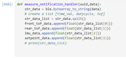
I then added functions on both the Jupyter notebook and robot, similar to previous labs, to transmit the collected data back to my laptop.

Python function to receive and record measured data:

Arduino function to transmit recorded ToF, IMU, and setpoint data:

Consider whether your robot behavior is reliable enough to assume that the readings are spaced equally in angular space, or if you are better off trusting the orientation from gyroscope values.

After recording and analyzing the received yaw data from the robot, I found the robot behavior to be reliable enough that the readings were spaced equally in angular space, as the robot settled within 5 degrees of each of the desired setpoints nicely. Thus, in future calculations, I utilized the commanded setpoint as the expected angle of the robot.

Sanity check individual turns by plotting them in polar coordinate plot. For simplicity assume that the robot is rotating in place. Do the measurements match up with what you expect?

To sanity check individual turns of the robot, I created the following polar plots at each of the 4 locations. As I had mounted ToF sensors on opposing sides of the robot, I was also able to check the repeatability of my measurements by comparing the front ToF sensor measurements with the rear ToF sensor measurements collected 180 degrees offset.

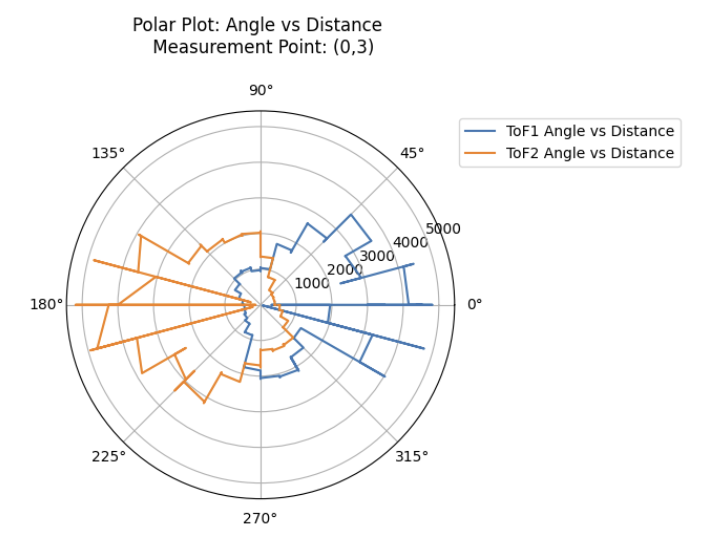
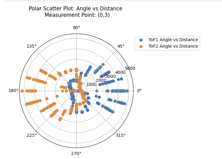
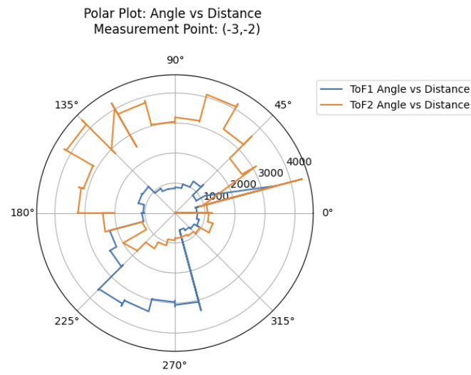
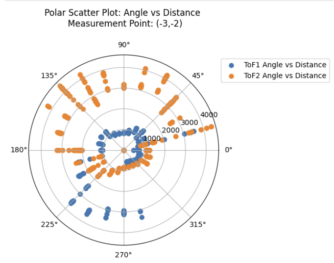
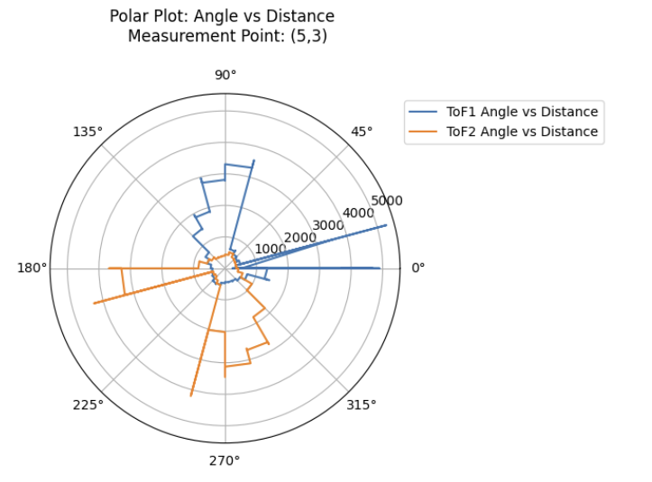
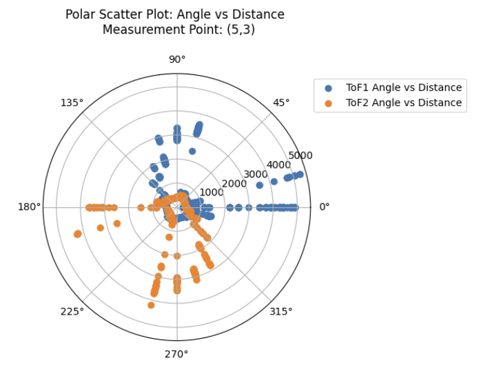
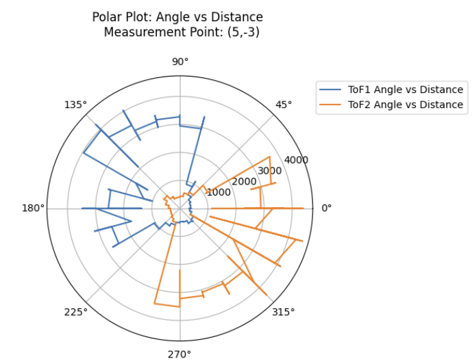
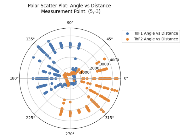
As can be seen in the plots above, the 2 ToF sensors corroborated each others' readings fairly well, with the exception of the measurements collected at (-3,-2). This was likely due to the overcorrection issue which was addressed earlier in the lab.

In that specific case, the ToF sensor readings from the front ToF sensor, ToF 2 , were completely inaccurate, which resulted in me just using ToF 1's readings for my future plots.

Compute the transformation matrices and convert the measurements from the distance sensor to the inertial reference frame of the room (these will depend on how you mounted your sensors on the robot.)

Next, we can use a 2D rotational transformation matrix to convert our Polar coordinates into Cartesian coordinates, to create a aggregate map of readings for the whole room.

Describe the matrices.

Using the transformation matrices described in Lecture 2, our rotational transformation matrix to apply to our 1 dimensional ToF readings is:

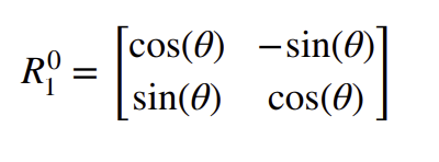
We can apply this rotation matrix using Jupyter notebook in the following implementation:

Essentially, we parse the received ToF data from the stored arrays, and apply the rotational transformation matrix to each reading. We also apply a linear transformation corresponding to the measurement location with respect to the origin. For example, in the snippet shown above, if measurements are taken at (0,3), we adjust the y coordinate of readings by 3 ft = 3*304mm. We additionally need to take into consideration that the sensors are located 180 degrees apart, so we need to apply a 180 degree or (pi radians) adjustment to the rear ToF sensor readings to bring them in line with the front ToF sensor readings.

As shown in the left hand side of the following generated plots, this code gives us an immense amount of noisy data points from the ToF sensors.

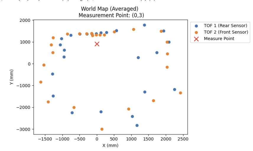
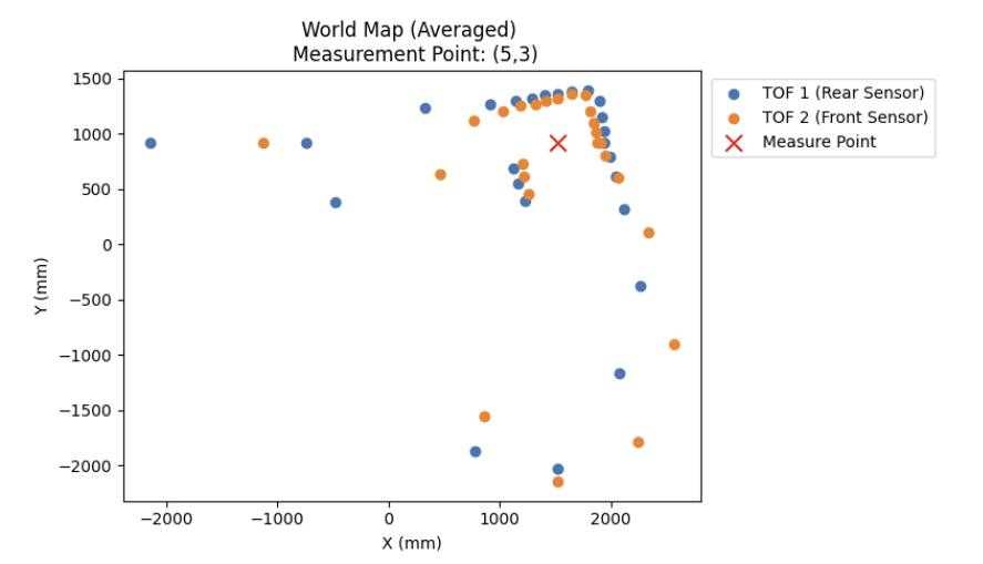
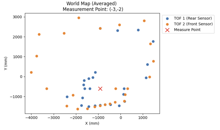
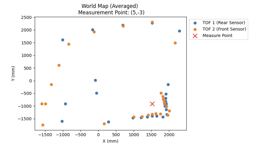
To counteract this, I wrote a script to iterate through each setpoint and take the average of the ToF readings at each setpoint, which resulted in the much cleaner plots shown on the right.

Plot all of your TOF sensor readings in a single plot. Please assign different colors to data sets acquired from each turn.

Combining all of the datapoints from the previously generated plots, I created a singular map and colored each of the datasets distinctly:

Lastly, using the world map created in Task 3, I manually fitted lines to the collected points, following the highest density point clusters.

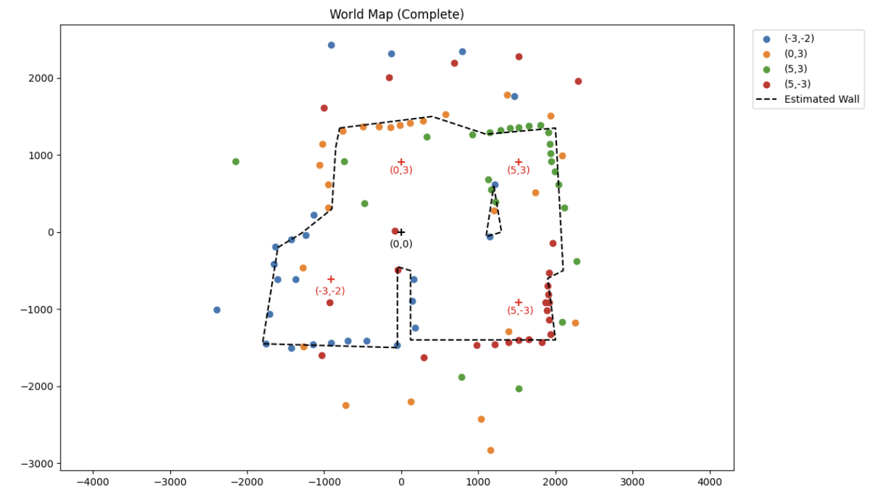
Additionally, to prepare for Lab 10, I created two lists containing the end points of the overlaid lines in the format (x_start, y_start) and (x_end, y_end).

I also wanted to see how closely my points aligned with the world map in reality.

Below is my robot's estimated map overlaid with the true world boundary:

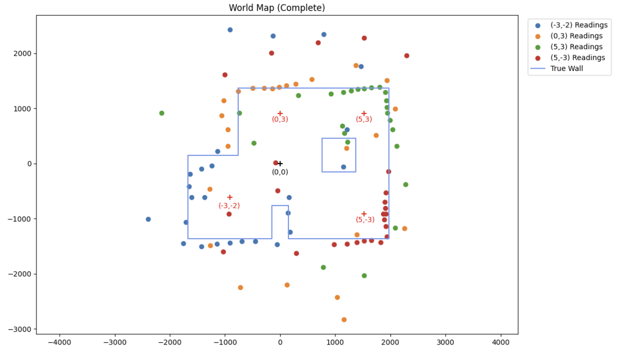
Overall, I think the data collected matched fairly well with the true boundary of the world with the exception of the square obstacle in the top right corner. For some reason, the entire left side of that obstacle failed to be mapped. One possible reason this could have happened is that the angular increments for my angular controller were so large that the robot missed the corner of the square obstacle in between turns, or overshot its distance resulting in points that were discarded as noise.

For future iterations, I would like to see how increasing the granularity of the angular increments of the mapping sequence would affect the resolution and accuracy of the resulting world map, as I suspect it might help to improve the detection of smaller obstacles like these.

Collaboration Statement

I referenced Nila Narayan's website for this lab.