Lab Tasks

Choose your step response, u(t), to be of similar size to the PWM value you used in Lab 5 (to keep the dynamics similar). Pick something between 50%-100% of the maximum u.

To begin this week's lab, I decided on a step response value that was similar to the PWM value I used in my Lab 5 testing. This way, the dynamics of the system would remain similar, ensuring that the constructed KF model would more closely reflect the behavior of the real-life system. As the majority of my testing had been conducted with a PWM value of 100, I selected a PWM value of 100 for this purpose.

Make sure your step time is long enough to reach steady state (you likely have to use active braking of the car to avoid crashing into the wall). Make sure to use a piece of foam to avoid hitting to wall and damaging your car.

Additionally, this step size of 100 was chosen to be just high enough to ensure I could reach a steady state velocity, but also short enough that it would allow me to track a sufficent amount of sensor data points before braking/hitting a wall.

Show graphs for the TOF sensor output, the (computed) speed, and the motor input. Please ensure that the x-axis is in seconds.

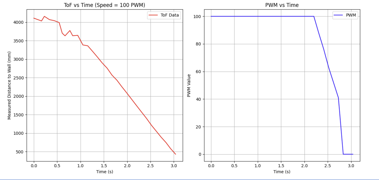
Using my PID controller code from Lab 5, I set the PWM limit of my controller to 100, and had the robot drive towards a wall to collect the following system data:

Measure the steady state speed, 90% rise time, and the speed at 90% rise time. (Note, this doesn't have to be 90% rise time. You could also use somewhere between 60-90%, but the speed and time must correspond to get an accurate estimate for m.)

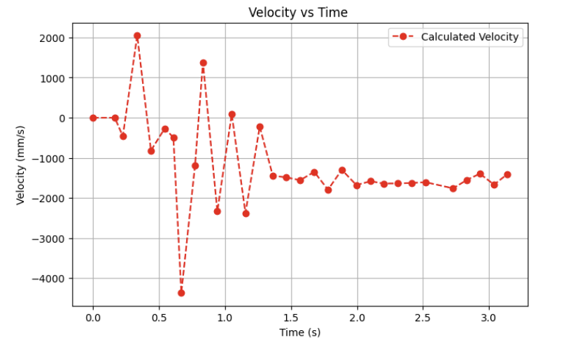
Although the collected data from the ToF was fairly noisy (as evidenced in the graphs above), I was able to make rough estimates for the following system parameters for the KF model:

Steady State Speed: 1.62 m/s.

90% Rise Time: 1.4 seconds.

Speed at 90% Rise Time: 1.458 m/s

I could then calculate the d and m terms using the following equations:

At steady state, we can approximate drag as \( d = \frac{u_{ss}}{\dot{x}_{ss}} \)

Thus, \( d = \frac{1N}{1.62 m/s} \approx 0.617 kg/s \)

And we can approximate momentum using the following equation derived from lecture: \[ m = -d \cdot \frac{t_r}{\ln(1 - d \cdot x_{ss})} \]

Substituting our values for d, \(t_r\) and \(x_{ss}\), we get

\[ m = -0.617 \cdot \frac{1.4}{\ln(1 - 0.9)} \approx .375 kg \]

When sending this data back to your laptop, make sure to save the data in a file so that you can use it even after your Jupyter kernel restarts.

Lastly, I saved all of my collected data from this test-run to a .csv file on my laptop for future use.

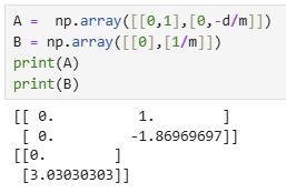
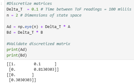
Compute the A and B matrix given the terms you found above, and discretize your matrices. Be sure to note the sampling time in your write-up.

Using the d and m terms I had calculated, I proceded with computing the A and B matrices for my system. Using our state space equations:

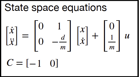
We can obtain and validate our A and B matrices:

And to discretize these matrices for our discrete ToF readings, we can use the sample rate of our ToF Sensors to obtain the following:

Identify your C matrix. Recall that C is a m x n matrix, where n are the dimensions in your state space, and m are the number of states you actually measure.

Then, we can initialize our C matrix, a 1 x 2 matrix, as our state space has 2 dimensions and we measure 1 state -- position:

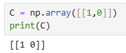
Note that our measured state has a positive coefficient as our measured ToF distances are all positive.

Initialize your state vector, x, e.g. like this: x = np.array([[-TOF[0]],[0]])

Then, I created an initial state vector which takes in our initial ToF sensor measurement (with a positive coefficient as I measured positive distance to the wall) and initial velocity (0 m/s).

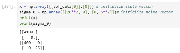
In this snippet, I also included my initialization for the initial noise vector, which describes our uncertainty in our initial state.

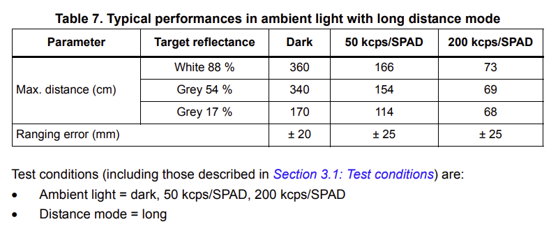
For our initial position noise, I referenced the +- 20mm ranging error value provided by the ToF sensor's datasheet:

As instructed, I also reasoned about a non-zero value for the velocity noise. Knowing that the error in our initial velocity being 0 m/s is practically 0 as the robot is at rest initially, (but could not be exactly 0 or the KF will not work) I instead chose an arbitrarily small value for variance of 25.

For the Kalman Filter to work well, you will need to specify your process noise and sensor noise covariance matrices.

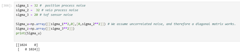
Lastly, to finalize my inputs for the KF, I needed to define parameters for process and measurement noise.

These parameters: \( \sigma_1 \), \( \sigma_2 \), and \( \sigma_3 \), represent the uncertainty in our modeled velocity , uncertainty in our modeled distance, and uncertainty in our measured ToF sensor readings respectively.

Using the process described in lecture, I calculated the values for \( \sigma_1 \), \( \sigma_2 \) using the sampling time of my sensor.

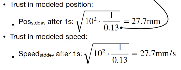
Substituting in a sampling time of .1s , we obtain a value of approximately 32 for \( \sigma_1 \) and \( \sigma_2 \) .

For \( \sigma_3 \), my sensor measurement noise, I used the sensor ranging error of 20mm in long distance mode as described previously from the datasheet.

These 3 parameters are then used to build the covariance matrices, 'Sigma_u' and 'Sigma_z'.

With all my inputs to the Kalman Filter finalized, I could then move on to test the filter on some sample ToF data in Jupyter Notebook.

Be sure to include a discussion of all the parameters that affect the performance of your filter.

In order to fine-tune my implementation for the Kalman Filter in simulation, I first wanted to explore how the various parameters to the KF affected the performance of the model.

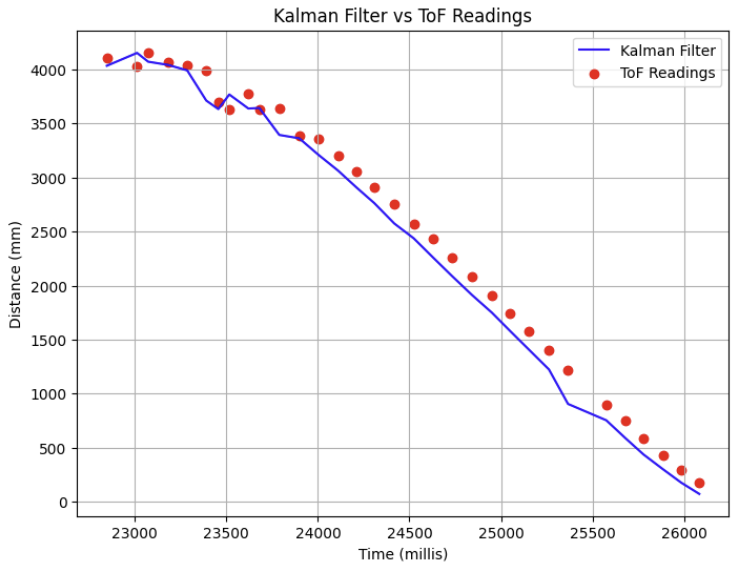
Increasing my values for \( \sigma_1 \) and \( \sigma_2 \) (parameters for process noise) will decrease my trust in the model, essentially placing more trust in the sensor readings.

As shown in the graph below, with arbitrarily large values of \( \sigma_1 \) and \( \sigma_2 \) = 100, and maintaining \( \sigma_3 \) = 20 we get a curve that closely resembles the ToF sensor readings (essentially overfitting to the collected data), albeit still slightly skewed from the actual ToF measurements.

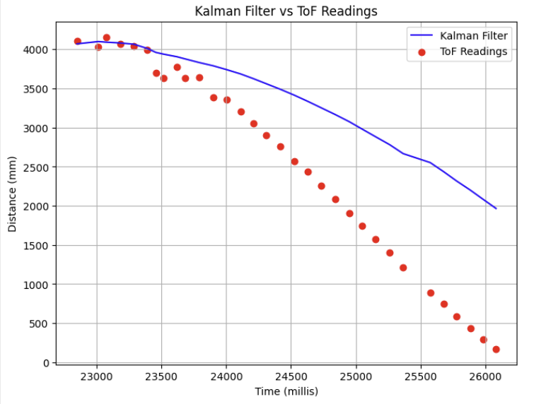
Alternatively, increasing my value for \( \sigma_3 \) (measurement noise) decreases my trust in the measured sensor readings and places more trust in my model.

As shown in the graph below, maintaining values for \( \sigma_1 \) and \( \sigma_2 \) at 22, and increasing my value for \( \sigma_3 \) = 100, we get a model output curve that is extremely skewed from the actual ToF readings.

Additionally, the output of the Kalman Filter is also dependent on the drag and momentum parameters that were derived from our system identification conducted at the beginning of this lab.

Ideally, a more rigorous and physically sound way of calculating these parameters for the system would result in a more accurate Kalman Filter than the estimation approach that I took in this lab.

Taking all of these factors into account, I applied my knowledge of these parameters to the collected ToF data from the initializing run and plotted the data using Matplotlib.

Plot the Kalman Filter output to demonstrate how well your Kalman Filter estimated the system state.

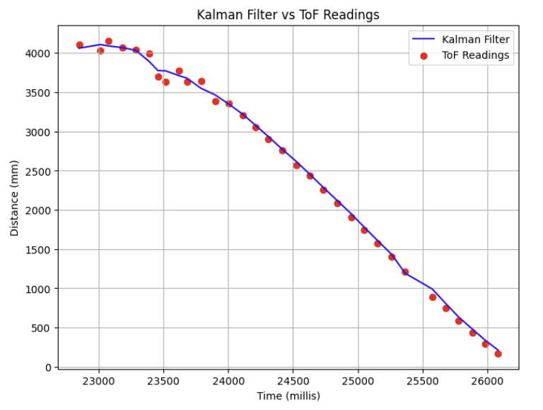
After some tweaking of parameters (as discussed above) we can see that the model fits the data that the system identification was performed on very well, as expected.

The final parameters used in this simulation were \( \sigma_1 \) and \( \sigma_2 \) = 22 , \( \sigma_3 \) = 20.

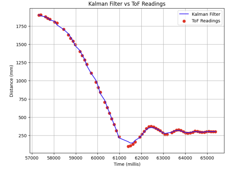
Additionally, I also wanted to test my Kalman Filter with the same parameters on a recorded run from Lab 5 with a different max PWM limit. In this trial, the max PWM was restrained to just 60.

Here were the results of that run:

If you have time, integrate the Kalman Filter into your Lab 5 PID solution on the Artemis. Before trying to increase the speed of your controller, use your debugging script to verify that your Kalman Filter works as expected.

Lastly, with the performance of the KF verified, I moved on to integrating the Kalman Filter on my robot.

The code to initialize the input parameters for the KF is shown below:

As much of the initialization and setup for the KF was a rewriting of the steps explained earlier for initializing the input parameters to the KF, I've added annotations directly to the code to clarify my methodology for brevity.

Below, I've also attached relevant annotated code snippet for the main PID control loop:

Important to highlight is that the Kalman Filter runs unconstrained from the sampling rate of the ToF sensor. When a new ToF data sample is not availble, the Kalman Filters' prediction step runs, updating the robot's known current distance.

And lastly, I've attached an annotated code snippet for the KF function that runs with each loop iteration:

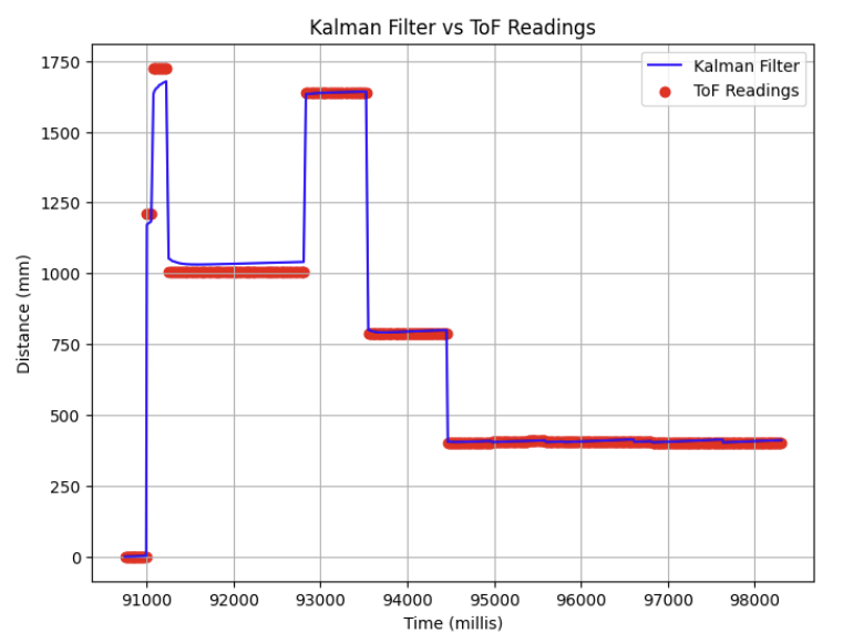
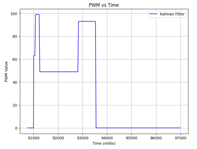
Using a max PWM limit of 100, I ran a PID test using the output of the Kalman Filter as the input to my proportional controller from Lab 5.

Be sure to demonstrate that your solution works by uploading videos and by plotting corresponding raw and estimated data in the same graph.

Here is a video of the results of the robot using the KF output as input to the P controller from Lab 5, successfully stopping within 1 foot of an obstacle:

And below is the data collected from the run:

Collaboration Statement

I referenced Nila Narayan and Mikayla Lahr's websites for this lab.